
This week’s BEACON Researchers at Work blog post is by MSU graduate student Matt Ryerkerk.
 A genetic algorithm is a method often used for optimization, or finding the best solution to a particular problem. When I first heard of genetic algorithms, I was working toward my Bachelors in Mechanical Engineering at MSU. Part of the senior capstone course included weekly guest lectures, the most memorable of which was a presentation by Dr. Ron Averill and Dr. Erik Goodman. They explained the basics of genetic algorithms and demonstrated how effective it could be when applied to engineering optimization problems. The work fascinated me enough that it was still on my mind several years later when I returned to MSU to pursue a PhD in Mechanical Engineering. Today I am lucky to be working with Dr. Averill and Dr. Goodman, along with Dr. Kalyanmoy Deb, on genetic algorithms.
Part of what drew me toward genetic algorithms, and optimization in general, is its multidisciplinary applications. Optimization is an important step of the design or decision process of any field. Even many day-to-day decisions can be thought to have gone through an optimization process. For example, when you go to school or work each morning there are a number of possible routes you can take. Each route will have different qualities, some will be shorter, some will be less busy, or some may be more scenic. The route that you choose is what you consider to be the most optimal route based on your preferences.
Optimization of engineering problems is not much different. Each problem will have a number of design variables that can be changed and criteria that should be met. For example, consider the design of a car body. You may want to ensure the crashworthiness of the car is as high as possible while also keeping the mass and cost of the body below a certain limit. The goal of the optimization method is to determine the values of the design variables that best meet this goal.
The idea of choosing an optimal solution from a set of all possible solutions is easily understood. However, what many people do not realize is that it is almost impossible to consider all possible solutions. If each possible solution needs to be evaluate—for example when designing the car—then each possible design would need to be run in a simulator in order to determine crashworthiness. A single design may contain tens, hundreds, or even thousands, of design variables. On top of that, each variable can have a large range of possible values. This is where the particular method of optimization comes in. Its job is to generate new, and hopefully better, solutions based on the information known. The measure of an optimization method is not just the quality of its best solutions but how many tries it took to get there.
There are many different types of optimization methods; depending on the problem some types will perform better than others. Genetic algorithms are optimization methods that take inspiration from natural selection. All organisms have their own DNA that controls their development and eventual traits. The organisms best fit for their environment will also be the most likely to survive and reproduce, passing their DNA on to the next generation.
Genetic algorithms operate in the same way. Each possible solution is given its own genome, just like how each organism has its own DNA. This genome contains all the design variables for that particular solution. This solution is evaluated (for example, by using the car crash simulator) and its performance is considered to be its “fitness.” The solutions with the best fitness will be used to recombine, or reproduce, with other solutions to produce new child solutions. The hope is that these children will perform better than either parent by combining the design traits that made them successful. Due to their simplicity, flexibility, and ease of operation, they are increasingly being used in many different optimization problems in sciences, engineering and commerce.
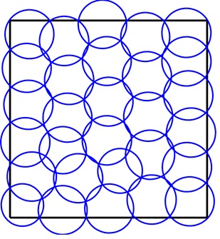
The placement and strength of the sensors (blue) are determined such that the cover the domain as efficiently as possible.
Our current work with genetic algorithms looks at a certain class of problems. Most problems contain a fixed number of design variables. Our work considers problems where the number of design variables may change from solution to solution. For example, one of our test problems involves placing sensors onto a field. Each sensor covers a circular area, we can control the position and sensing radius of each sensor. We want to cover the field as extensively as possible while minimizing the total cost of the sensors. The size of the genome will be different for solutions that contain different numbers of sensors. This introduces new questions of how to recombine solutions to produce offspring solutions; genetic algorithms typically only consider genomes of a fixed length.
Using traditional genetic algorithm methods for recombination almost always fails to produce children with finesses similar to that of the parents. What we’ve found is that additional care needs to be taken when exchanging information between the two parent solutions. First, parts of the two parent genomes that perform similar functions should be identified. In the sensor placement problem, for example, sensors that cover similar regions of the field in parent solutions should be identified. Using this information allows for a more controlled recombination of parent solutions and can reliably produce quality children, even when the parents contain different numbers of design variables.
Additionally, we’ve found that to produce solutions with the optimal number of sensors we have to try to protect solutions that contain a different numbers of sensors than their peers. For example, all possible solutions up until a point in the optimization run might contain 30 or more sensors. If a solution appears that contains only 29 sensors it is likely to be considered a poor solution as it will likely leave a portion of the field uncovered. However, 29 sensors may be closer to the optimal number of sensors. By giving these solutions some additional time to improve themselves, we may find that they will be the most optimal in the end, even if they perform poorly in the beginning.
For more information about Matt’s work, you can contact him at matt dot ryerkerk at gmail dot com.
