
This blog post was written by students in BEACON’s Fall 2013 Computational Science for Evolutionary Biologists course, taught by MSU faculty Titus Brown and graduate student Randy Olson. Blog post lead author: S. Kevin McCormick, with contributions from Zach Laubach, Nicolas Schmelling, Josephine Wee, and Phillip Brooks.
Ever wanted to play “god”? Perhaps, create a world and place some simple organisms on it to see what develops. You could surely answer a lot of questions about the beauty and diversity that has evolved on this planet. Some of our own have actually managed to run long term experiments on fast replicating organisms to do just that. However, that’s not exactly possible when one is working with longer living animals, or most other living organisms for that matter.
Another option would be to create artificial life forms that live and evolve within a digitally created world. This is not science fiction: computer models allowing scientists to test how populations of organisms react to change started popping up decades ago. Now labs are creating digital organisms with “DNA code” that can replicate, mutate, and evolve under any scenario that computer scientists and biologists can cook up. During Michigan State University’s CSE 801 course, run through the BEACON program, graduate students are introduced to a few of these computer models. One is a digital optimal foraging model called Area Restricted Search (ARS). The ARS model is based on a genetic algorithm that allows researchers to create a population of organisms with a few simple traits that can mutate over successive generations. These populations of organisms are placed in a world with a resource type, and given an award of higher fitness if they can find the resources. Natural selection can then act upon the population by giving preferential replication to the organisms with higher fitness.
Our class was first taught how to create digital populations that both did and did not evolve ARS strategies to find resources. We accomplished these tasks by allowing for trait changes in turning angle when in contact or away from resources, and the memory to turn in those situations, after each successive generation. Typically, when resources were sparsely and randomly distributed, an ARS strategy evolved quickly. Organisms turned more when in contact with food, turned less off food, and memory capacity increased. However, when resources were ubiquitous through the environment, ARS did not evolve, or evolved very slowly. For our class’s final project, we were asked to take the code for the ARS model, and manipulate it to answer evolutionary questions we were interested in. Our group wanted to see if we could evolve different ARS strategies in populations that were allopatrically isolated in environments with different resource types. If this was possible, we then wished to determine if the different ARS strategies of these populations gave advantages to a particular population when introduced to an environment with different resources. We hoped to use this as a model for testing questions about indirect competition.
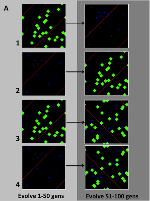
Figure 1: Example of environmental switching. Blue = small valuable resources, Green = large low value resources.
We began by manipulating the IPython code to create different resource environments that could change at a time our choosing. The environments themselves are made of digital grids, called ipythonblocks, where resources are distributed randomly over each successive generation. We altered the code to allow for multiple resource types of different size, value, and presence in the environment. We then created four simulations to test if allopatrically isolated populations evolved different ARS strategies, which could give one population an advantage when introduced to its “competitors” environment, or to environment of mixed resources (Figure 1). Each population (30 individuals) was first allowed to evolve for 50 generations on either rare small high-value resources, or large common low-value resources, at a trait mutation rate of 0.01 per generation. Then these populations were switched onto a new resource environment and allowed to evolve for another 50 generations under the same mutation rate. These simulations were run through EC2 instances on Amazon mainframes, and each took only 8 hours to complete.
Unfortunately, this first experiment did not work as planned. Separate ARS strategies and traits never evolved to fixation, and limitations in our code led to treatment effects in our separate environments (Figures 2 & 3). Most notably we ended up doubling resources when we created mixed resource environments, and we may not have allowed for enough time for separate ARS strategies to evolve. Therefore, because we were allowed another week, we chose to extend our model and fiddle with our created worlds and organisms a little more.
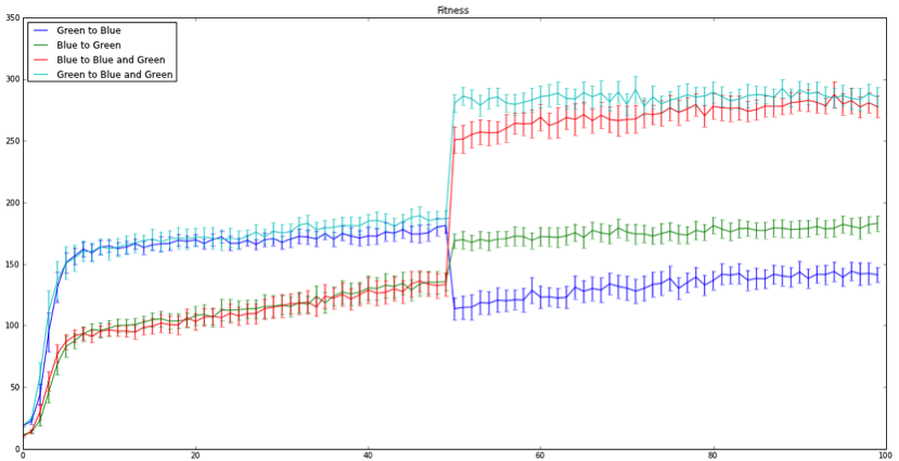
Figure 2: Fitness level over 100 generations. Shift at 50 generations reflects switching each population’s environment. Lines represent each individual population mean. Bars represent 95% confidence intervals.
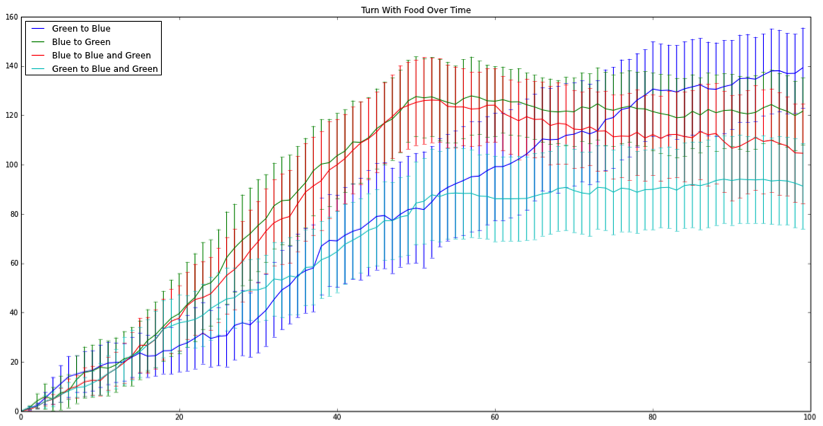
Figure 3: Turn angle increase when encountering food over 100 generation. Lines represent each individual population mean. Bars represent 95% confidence intervals.
First we created worlds where opportunities to increase fitness were equal in all aspects except for the ability to find the resources. Then we ran simulations we previously did not have time for, including evolving populations on mixed resources and switching them onto monocultures, as well as evolving populations solely on one type of resource base as controls. Next we allowed populations to persist for additional generations before switching resource environments.
Looking back now, I think that this may have been enough, but it seemed that the power to create and modify our little worlds with a few more lines of code may have gone to our heads. We chose to increase the mutation rate 10 fold prior to the environment shift, thinking that it would allow for a greater chance of different ARS strategies to evolve in the time we had. We then went even farther and stopped mutation just prior to the environment shifts. It was our hope that, if different ARS strategies did evolve to fixation, populations would be forced to use their evolved strategy in their new environment without the possibility of evolving a new one. Ideally this would artificially reflect wha
t is occasionally seen when generalist foragers invade new environments, and when specialist populations are displaced into new environments.
Unfortunately that last code change to the mutation rate was just a bit too much. By increasing the mutation rate tenfold we allowed for trait changes to jump all over the place for each successive generation. As Randy said, “we more or less eliminated inheritance,” as each individual lineage could drop or increase in trait changes at a rate higher than the code could allow for fitness increases. Therefore, there was no way for natural selection to properly act upon the population, perhaps some individual lineages, but not the population. This can be seen in Figure 4, when we shut off mutation at 60 generations, because afterward we observed what appeared to be population sorting. Following the mutation shutoff, individuals within the population with “better” trait values started to out-compete their relatives.
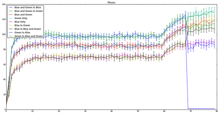
Figure 4: Fitness level over 100 generations. Lines represent each individual population mean. Bars represent 95% confidence intervals. Note: the blue line drop just before 70 generations reflects a coding error.
It seemed that everything we did to try to create different ARS strategies had the opposite effect. All traits, averaged across each population, ended up at the same level prior to the mutation shutoff, and the only significant difference we observed was different levels of fitness for each resource environment. It seems that playing “god” is a bit more difficult than we thought. However, thanks to this course we now have a better understanding of what it takes to create digital organisms and worlds, as well as how complicated it can be to model evolution. In the future we hope to extend these models to allow for other drivers of evolution, such as direct competition, death, energy expenditure, stochastic resource availability, evolution of different traits…….
